Hands-on tutorials - Fourier Neural Operator for 1D Burgers equation#
Author: Xiaoyu Xie
Date: May 25, 2024
What is Fourier Neural Operator?#
Fourier Neural Operator (FNO) {cite}li2020fourier is one of the most popular operator learning approach for solving Partial Differential Equations (PDEs) using data.
From the machine learning perspective, FNO is just a combination of three main steps:
(1) Lifting the channel dimension,
(2) FNO block (using truncated and linear transformed fourier mode to learn non-local/global features + using 1*1 Conv to learn local features and make sure the Conv can deal with different resolution),
(3) Reducing the channel dimension to the desired output dimension.
from IPython.display import YouTubeVideo
YouTubeVideo('Rb8GyyTDlTc', width=700, height=400)
How to implement FNO?#
from IPython.display import YouTubeVideo
YouTubeVideo('Syf0RNt3EkM', width=700, height=400)
Download dataset#
Important notes:
Make sure you download and save the dataset from (https://drive.google.com/file/d/1tsSyxcSSKkQ2SWsSpId8s5bKFgbn8boI/view?usp=sharing) to your google drive or your local computer
Make sure you choose GPU in the Runtime/Change runtime type or use GPU in your local computer
import os
from google.colab import drive
import warnings

warnings.filterwarnings('ignore')

def is_running_on_colab():
    return 'COLAB_GPU' in os.environ

# Use the function to check
if is_running_on_colab():
    print("This notebook is running on Google Colab.")

    # Mount your Google Drive.
    drive.mount("/content/drive")

    # check whether the dataset is already in your google drive or local computer
    # make sure burgers_data_R10.mat is in this folder of your google drive
    !ls /content/drive/MyDrive/Dataset

    # used for Colab. You need to change the path for your file
    dataset_path = '/content/drive/MyDrive/Dataset/burgers_data_R10.mat'
else:
    print("This notebook is not running on Google Colab.")
    dataset_path = 'dataset/burgers_data_R10.mat' # put the dataset in a relative path
Import python packages#
import os

import matplotlib.pyplot as plt
import numpy as np
import pytorch_lightning as pl
from pytorch_lightning.callbacks import ModelCheckpoint
from pytorch_lightning import seed_everything
from scipy.io import loadmat
import torch
import torch.nn as nn
import torch.nn.functional as F
from torch.utils.data import DataLoader, TensorDataset
System configuration#
# set random seed for reproducibility
seed_everything(seed=0)
torch.backends.cudnn.deterministic = True
torch.backends.cudnn.benchmark = False

# choose a specific GPU ID
os.environ['CUDA_VISIBLE_DEVICES'] = '1'
device = torch.device(f'cuda' if torch.cuda.is_available() else 'cpu')

# print pytorch version and cuda version
print(torch.__version__)
Global seed set to 0
1.13.0+cu116
Define FNO model#
class SpectralConv1d(nn.Module):
    """
    Spectral Convolutional 1D Layer.

    Args:
        in_channels (int): Number of input channels.
        out_channels (int): Number of output channels.
        modes1 (int): Number of Fourier modes to multiply, at most floor(N/2) + 1.

    Attributes:
        in_channels (int): Number of input channels.
        out_channels (int): Number of output channels.
        modes1 (int): Number of Fourier modes to multiply, at most floor(N/2) + 1.
        scale (float): Scaling factor for the weights.
        weights1 (nn.Parameter): Learnable weights for the convolution.

    Methods:
        compl_mul1d(input, weights): Performs complex multiplication between input and weights.
        forward(x): Forward pass of the SpectralConv1d layer.
    """

    def __init__(self, in_channels, out_channels, modes1):
        super(SpectralConv1d, self).__init__()
        self.in_channels = in_channels
        self.out_channels = out_channels
        self.modes1 = modes1  # Number of Fourier modes are kept, at most floor(N/2) + 1

        self.scale = 1 / (in_channels * out_channels)
        self.weights1 = nn.Parameter(self.scale * torch.rand(in_channels, out_channels, self.modes1, dtype=torch.cfloat))

    def compl_mul1d(self, input, weights):
        """
        Performs complex multiplication between input and weights.

        Args:
            input (torch.Tensor): Input tensor of shape (batch, in_channel, x).
            weights (torch.Tensor): Weights tensor of shape (in_channel, out_channel, x).

        Returns:
            torch.Tensor: Result of complex multiplication of input and weights, of shape (batch, out_channel, x).
        """
        # (batch, in_channel, x ), (in_channel, out_channel, x) -> (batch, out_channel, x)
        # in_channel is the common dimension along which the operation is performed.
        # It suggests that every channel (or feature) of the input is being transformed into a new set of channels (or features) in the output.
        # The operation iterates over each batch and each position x, multiplying the input channels
        # by the corresponding weights and summing the results to produce the output channels.

        # For a given position i in the x dimension and a given batch element:
        # Take all values in A at this position and batch (A[batch, :, i]) – a slice of shape (in_channel).
        # Take all corresponding values in B at this position (B[:, :, i]) – a matrix of shape (in_channel, out_channel).
        # Multiply these values element-wise and sum over the in_channel dimension.
        # This produces a vector of shape (out_channel), representing the transformed features at position i for this batch element.
        return torch.einsum("bix,iox->box", input, weights)

    def forward(self, x):
        # Compute Fourier coeffcients
        x_ft = torch.fft.rfft(x)  # [Batch, C_in, Nx] -> [Batch, C_in, Nx//2 + 1], eg. [20, 64, 128] -> [20, 64, 65]

        # Multiply relevant Fourier modes
        out_ft = torch.zeros(x.shape[0], self.out_channels, x.size(-1)//2 + 1,  device=x.device, dtype=torch.cfloat) # [Batch, Nc, Nx//2 + 1], eg. [20, 64, 65]
        # [Batch, C_in, self.modes1] * [C_in, C_out, self.modes1] -> [Batch, C_out, self.modes1]
        out_ft[:, :, :self.modes1] = self.compl_mul1d(x_ft[:, :, :self.modes1], self.weights1)

        # Return to physical space
        x = torch.fft.irfft(out_ft, n=x.size(-1))  # [Batch, C_out, self.modes1] -> [Batch, C_out, Nx], eg. [20, 64, 65] -> [20, 64, 128]
        return x

class FNO1d(nn.Module):
    def __init__(self, modes, width):
        """
        1D Fourier Neural Operator model.

        Args:
            modes (int): Number of spectral modes.
            width (int): Number of hidden channel.
        """
        super(FNO1d, self).__init__()
        self.modes1 = modes
        self.width = width
        self.fc0 = nn.Linear(2, self.width) # input channel is 2: (a(x), x) MeshgridTensor + initial condition

        self.conv0 = SpectralConv1d(self.width, self.width, self.modes1)
        self.conv1 = SpectralConv1d(self.width, self.width, self.modes1)
        self.conv2 = SpectralConv1d(self.width, self.width, self.modes1)
        self.conv3 = SpectralConv1d(self.width, self.width, self.modes1)

        self.w0 = nn.Conv1d(self.width, self.width, 1)
        self.w1 = nn.Conv1d(self.width, self.width, 1)
        self.w2 = nn.Conv1d(self.width, self.width, 1)
        self.w3 = nn.Conv1d(self.width, self.width, 1)

        self.fc1 = nn.Linear(self.width, 128)
        self.fc2 = nn.Linear(128, 1)

    def forward(self, x):
        # stage 1: lift the channel from 2 to self.width = 64
        x = self.fc0(x)         # [Batch, Nx, C] -> [Batch, Nx, Width], eg. [20, 128, 2] -> [20, 128, 64]
        x = x.permute(0, 2, 1)  # [Batch, C, Nx], eg. [20, 64, 128]

        # stage 2: integral operators u' = (W + K)(u).
        # W is the linear transformation; K is the spectral convolution kernel.
        x1 = self.conv0(x)      # [Batch, C, Nx], eg. [20, 64, 128]
        x2 = self.w0(x)         # [Batch, C, Nx], eg. [20, 64, 128]
        x = x1 + x2
        x = F.relu(x)           # [Batch, C, Nx], eg. [20, 64, 128]

        x1 = self.conv1(x)
        x2 = self.w1(x)
        x = x1 + x2
        x = F.relu(x)           # [Batch, C, Nx], eg. [20, 64, 128]

        x1 = self.conv2(x)
        x2 = self.w2(x)
        x = x1 + x2
        x = F.relu(x)           # [Batch, C, Nx], eg. [20, 64, 128]

        x1 = self.conv3(x)
        x2 = self.w3(x)
        x = x1 + x2             # [Batch, C, Nx], eg. [20, 64, 128]

        # stage 3: put the channel back to 1
        x = x.permute(0, 2, 1)  # [Batch, Nx, C], eg. [20, 128, 64]
        x = self.fc1(x)         # [Batch, Nx, C] -> [Batch, Nx, 128], eg. [20, 128, 64] -> [20, 128, 128]
        x = F.relu(x)
        x = self.fc2(x)         # [Batch, Nx, C] -> [Batch, Nx, 1], eg. [20, 128, 128] -> [20, 128, 1]

        # since there are only one output
        x = x.squeeze(-1)       # [Batch, Nx, 1] -> [Batch, Nx], eg. [20, 128, 1] -> [20, 128]

        return x
Configuration#
class Config():
    #========================#
    # Training parameters
    #========================#
    # num_epoch = 500                  # number of training epoch
    num_epoch = 20                 # for debugging
    batch_size = 20                  # batch size

    # Adam optimizer parameters
    weight_decay = 1e-4              # weight decay for Adam optimizer

    # learning rate decay parameters
    lr = 0.001                       # learning rate
    step_size = 100                  # step size for step-wise learning rate decay
    gamma = 0.5                      # the decay coefficient for step-wise learning rate decay

    modes = 16                       # number of Fourier modes to multiply, at most floor(N/2) + 1
    width = 64                       # number of hidden channel

    #========================#
    # dataset information
    #========================#
    # download dataset from: https://drive.google.com/file/d/16a8od4vidbiNR3WtaBPCSZ0T3moxjhYe/view?usp=drive_link
    dataset_path = 'dataset/burgers_data_R10.mat'
    sub = 8                             # downsample rate for spatial dimension
    resolution_original = 2**13         # original resolution of the dataset
    num_train = 1000                    # number of training data
    num_test = 200                      # number of test data

    #========================#
    # results
    #========================#
    model_path = 'results/model_burgers_R10'
    checkpoint_dir = 'results/checkpoints_burgers_R10'

cfg = Config()
Dataset preparation#
def prepare_data(raw_data, sub, cfg):
    """
    Load raw data and prepare data loaders.
    """
    x_data = torch.Tensor(raw_data['a'])[:, ::sub]  # (num_trajectory, Nx): (2048, 1024)
    y_data = torch.Tensor(raw_data['u'])[:, ::sub]  # (num_trajectory, Nx): (2048, 1024)
    print(f'[Dataset] downsampled raw data - x_data: {x_data.shape}, y_data: {y_data.shape}')

    # Split into train and test
    x_train, y_train = x_data[:cfg.num_train, :], y_data[:cfg.num_train, :]
    x_test, y_test = x_data[-cfg.num_test:, :], y_data[-cfg.num_test:, :]
    print(f'[Dataset] x_train: {x_train.shape}, y_train: {y_train.shape}')
    print(f'[Dataset] x_test: {x_test.shape}, y_test: {y_test.shape}')

    # Prepare grid information (optional)
    grid_all = np.linspace(0, 1, cfg.resolution_original).reshape(cfg.resolution_original, 1).astype(np.float64)
    grid = grid_all[::sub, :]
    grid = torch.tensor(grid, dtype=torch.float)

    # Concatenate the spatial grid and the spatial solution
    x_train = torch.cat([x_train.reshape(cfg.num_train, -1, 1), grid.repeat(cfg.num_train, 1, 1)], dim=2)
    x_test = torch.cat([x_test.reshape(cfg.num_test, -1, 1), grid.repeat(cfg.num_test, 1, 1)], dim=2)

    # Create data loaders
    train_loader = DataLoader(TensorDataset(x_train, y_train), batch_size=cfg.batch_size, shuffle=True)
    test_loader = DataLoader(TensorDataset(x_test, y_test), batch_size=cfg.batch_size, shuffle=False)

    return train_loader, test_loader

class DataModule(pl.LightningDataModule):
    """
    Data module for loading data in PyTorch Lightning.
    """
    def __init__(self, dataset_path, sub, cfg):
        super(DataModule, self).__init__()
        self.dataset_path = dataset_path
        self.sub = sub
        self.cfg = cfg
        self.train_loader = None
        self.test_loader = None

    def setup(self, stage=None):
        # Load training data
        raw_data = loadmat(self.dataset_path)  # Load data as a dictionary
        self.train_loader, self.test_loader = prepare_data(raw_data, self.sub, self.cfg)
        print('[DataModule] Data loaders have been set up.')

    def train_dataloader(self):
        return self.train_loader

    def val_dataloader(self):
        return self.test_loader

    def test_dataloader(self):
        return self.test_loader

data_module = DataModule(cfg.dataset_path, cfg.sub, cfg)
data_module.setup()
[Dataset] downsampled raw data - x_data: torch.Size([2048, 1024]), y_data: torch.Size([2048, 1024])
[Dataset] x_train: torch.Size([1000, 1024]), y_train: torch.Size([1000, 1024])
[Dataset] x_test: torch.Size([200, 1024]), y_test: torch.Size([200, 1024])
[DataModule] Data loaders have been set up.
Model training & evaluation#
class PlModel(pl.LightningModule):
    """
    PyTorch Lightning module for training the FNO model.
    """
    def __init__(self, cfg):
        super(PlModel, self).__init__()
        self.model = FNO1d(cfg.modes, cfg.width)
        self.cfg = cfg
        self.metrics = {'train_loss': [], 'val_loss': [], 'test_loss': []}

    def forward(self, x):
        return self.model(x)

    def training_step(self, batch, batch_idx):
        x, y = batch
        y_hat = self.model(x)
        loss = F.mse_loss(y_hat.view(-1, 1), y.view(-1, 1))
        self.log('train_loss', loss, on_step=False, on_epoch=True, prog_bar=True, logger=True)
        self.metrics['train_loss'].append(loss.item())
        return loss

    def validation_step(self, batch, batch_idx):
        x, y = batch
        y_hat = self.model(x)
        loss = F.mse_loss(y_hat.view(-1, 1), y.view(-1, 1))
        self.log('val_loss', loss, on_step=False, on_epoch=True, prog_bar=True, logger=True)
        self.metrics['val_loss'].append(loss.item())
        return loss

    def test_step(self, batch, batch_idx):
        x, y = batch
        y_hat = self.model(x)
        loss = F.mse_loss(y_hat.view(-1, 1), y.view(-1, 1))
        self.log('test_loss', loss, on_step=False, on_epoch=True, prog_bar=True, logger=True)
        self.metrics['test_loss'].append(loss.item())
        return loss

    def configure_optimizers(self):
        optimizer = torch.optim.Adam(self.model.parameters(), lr=self.cfg.lr, weight_decay=self.cfg.weight_decay)
        scheduler = torch.optim.lr_scheduler.StepLR(optimizer, step_size=self.cfg.step_size, gamma=self.cfg.gamma)
        return [optimizer], [scheduler]

    def evaluate_at_different_resolutions(self, raw_data, resolution_test_list):
        for resolution_test in resolution_test_list:
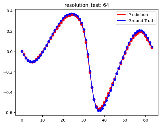
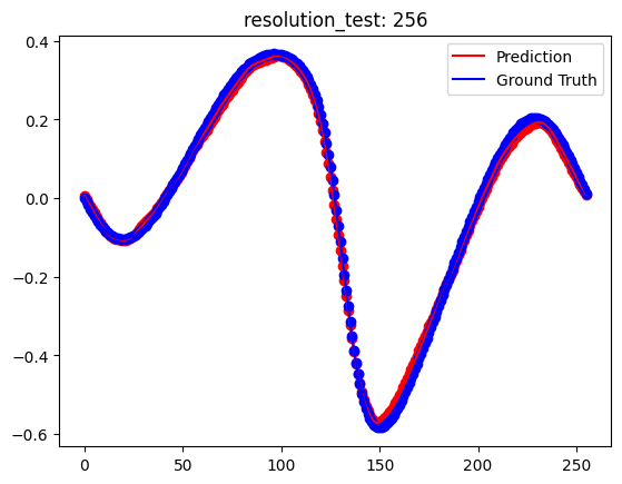
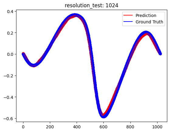
            print('[Test] resolution_test: ', resolution_test)
            sub = self.cfg.resolution_original // resolution_test
            _, test_loader = prepare_data(raw_data, sub, self.cfg)

            self.eval()
            with torch.no_grad():
                for x, y in test_loader:
                    x, y = x.to(self.device), y.to(self.device)
                    pred = self(x)

                    # Plot comparison for the first example in the batch
                    plt.figure()
                    plt.plot(pred[0].cpu().numpy(), 'r', label='Prediction')
                    plt.plot(y[0].cpu().numpy(), 'b', label='Ground Truth')
                    plt.scatter(np.arange(resolution_test), pred[0].cpu().numpy(), c='r')
                    plt.scatter(np.arange(resolution_test), y[0].cpu().numpy(), c='b')
                    plt.legend(loc='upper right')
                    plt.title(f'resolution_test: {resolution_test}')
                    plt.show()

                    # only plot the first batch
                    break
# train the model
model = PlModel(cfg)

checkpoint_callback = ModelCheckpoint(
    monitor='val_loss',
    dirpath=cfg.checkpoint_dir,
    filename='fno-{epoch:02d}-{val_loss:.2f}',
    save_top_k=1,
    mode='min',
)

trainer = pl.Trainer(
    max_epochs=cfg.num_epoch,
    callbacks=[checkpoint_callback],
    accelerator='gpu',
    devices=1,
    enable_progress_bar=False,
    # Note: I disabled progress bar to make the ouput cell
    # more clear for jupyter notebook. But it's better to enable it for python script.
)
# train the model
trainer.fit(model, data_module)
# test the model
trainer.test(model, data_module.test_dataloader())

# Evaluate the model at different resolutions
raw_data = loadmat(cfg.dataset_path)  # Ensure this is loaded correctly
resolution_test_list = [64, 256, 1024]
model.evaluate_at_different_resolutions(raw_data, resolution_test_list)
GPU available: True (cuda), used: True
TPU available: False, using: 0 TPU cores
IPU available: False, using: 0 IPUs
HPU available: False, using: 0 HPUs
You are using a CUDA device ('NVIDIA RTX A6000') that has Tensor Cores. To properly utilize them, you should set `torch.set_float32_matmul_precision('medium' | 'high')` which will trade-off precision for performance. For more details, read https://pytorch.org/docs/stable/generated/torch.set_float32_matmul_precision.html#torch.set_float32_matmul_precision
[Dataset] downsampled raw data - x_data: torch.Size([2048, 1024]), y_data: torch.Size([2048, 1024])
[Dataset] x_train: torch.Size([1000, 1024]), y_train: torch.Size([1000, 1024])
[Dataset] x_test: torch.Size([200, 1024]), y_test: torch.Size([200, 1024])
[DataModule] Data loaders have been set up.
LOCAL_RANK: 0 - CUDA_VISIBLE_DEVICES: [1]

  | Name  | Type  | Params
--------------------------------
0 | model | FNO1d | 287 K
--------------------------------
287 K     Trainable params
0         Non-trainable params
287 K     Total params
1.150     Total estimated model params size (MB)
`Trainer.fit` stopped: `max_epochs=20` reached.
LOCAL_RANK: 0 - CUDA_VISIBLE_DEVICES: [1]
[Dataset] downsampled raw data - x_data: torch.Size([2048, 1024]), y_data: torch.Size([2048, 1024])
[Dataset] x_train: torch.Size([1000, 1024]), y_train: torch.Size([1000, 1024])
[Dataset] x_test: torch.Size([200, 1024]), y_test: torch.Size([200, 1024])
[DataModule] Data loaders have been set up.
────────────────────────────────────────────────────────────────────────────────────────────────────────────────────────
       Test metric             DataLoader 0
────────────────────────────────────────────────────────────────────────────────────────────────────────────────────────
        test_loss         0.00026296277064830065
────────────────────────────────────────────────────────────────────────────────────────────────────────────────────────
[Test] resolution_test:  64
[Dataset] downsampled raw data - x_data: torch.Size([2048, 64]), y_data: torch.Size([2048, 64])
[Dataset] x_train: torch.Size([1000, 64]), y_train: torch.Size([1000, 64])
[Dataset] x_test: torch.Size([200, 64]), y_test: torch.Size([200, 64])

[Test] resolution_test:  256
[Dataset] downsampled raw data - x_data: torch.Size([2048, 256]), y_data: torch.Size([2048, 256])
[Dataset] x_train: torch.Size([1000, 256]), y_train: torch.Size([1000, 256])
[Dataset] x_test: torch.Size([200, 256]), y_test: torch.Size([200, 256])

[Test] resolution_test:  1024
[Dataset] downsampled raw data - x_data: torch.Size([2048, 1024]), y_data: torch.Size([2048, 1024])
[Dataset] x_train: torch.Size([1000, 1024]), y_train: torch.Size([1000, 1024])
[Dataset] x_test: torch.Size([200, 1024]), y_test: torch.Size([200, 1024])

Plot training and validation loss#
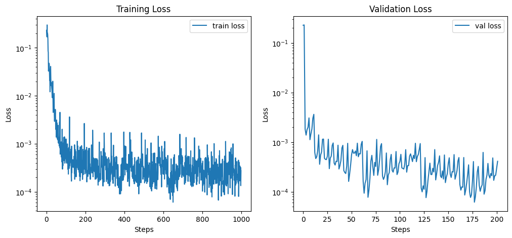
# plot the training loss and validation loss in two subplots
plt.figure(figsize=(12, 5))
plt.subplot(1, 2, 1)
plt.plot(model.metrics['train_loss'], label='train loss')
plt.xlabel('Steps')
plt.ylabel('Loss')
plt.yscale('log')
plt.title('Training Loss')
plt.legend()

plt.subplot(1, 2, 2)
plt.plot(model.metrics['val_loss'], label='val loss')
plt.xlabel('Steps')
plt.ylabel('Loss')
plt.yscale('log')
plt.title('Validation Loss')
plt.legend()
plt.show()

Homework#
To get better performance, you can increase num_epoch to 500 and train the model again. You will see the loss can be much smaller.
You can also use other techniques, such as different batch sizes or learning rates or learning rate decay schemes to get better performance.
Reference#
FNO paper: Li, Z., Kovachki, N., Azizzadenesheli, K., Liu, B., Bhattacharya, K., Stuart, A., & Anandkumar, A. (2020). Fourier neural operator for parametric partial differential equations. arXiv preprint arXiv:2010.08895
FNO official github: neuraloperator/neuraloperator
FNO tutorial: Ceyron/machine-learning-and-simulation
DeepONet & FNO: lu-group/deeponet-fno
FNO documentation: https://neuraloperator.github.io/neuraloperator/dev/user_guide/neural_operators.html
FNO blog: https://zongyi-li.github.io/blog/2020/fourier-pde/
Julia: https://docs.sciml.ai/NeuralOperators/stable/introduction/
Citation#
If you find this tutorial helpful, please cite it:
@book{xie2024sml,
  title={Hands-on Scientific Machine Learning},
  author={Xiaoyu Xie},
  url={https://xiaoyuxie.top/Sci-ML-Book},
  year={2024},
  publisher={WWW}
}
